Mapping Pollen Allergens for the Whole Earth

A single WebGL map that lets you pick the allergens that affect you and scrub a 52-week timeline anywhere on Earth. The hard part is not the rendering — it is doing this honestly when measured pollen data exists for only a handful of regions. Here is exactly how each pixel is sourced, modelled, and labelled.

Open the interactive map →

What data we use, and where

Every pixel on the map comes from one of three kinds of source, and the kind decides how much you can trust it. Think of it as a precision hierarchy — from real airborne-pollen measurements down to a season computed from satellite and climate data:

Highest precision — measured station networks. Two regions are anchored on real airborne-pollen measurements. Europe comes from the EAN [European Aeroallergen Network] climatology, published as the ContaminationMapEurope widget on polleninformation.at. The US (CONUS) [contiguous United States] comes from PECM 2.0 [Pollen Emissions for Climate Models] — a 1995–2014 measured pollen-emission climatology (Zhang & Steiner 2022). We download each, decode it to weekly pollen levels, and spatially interpolate between stations.
Medium precision — literature & monitoring-network calendars. The other populated regions — East Asia, Oceania (via the TERN/ACEAS [Australian ecology monitoring network]), the Middle East, the rest of Asia, Latin America, and Africa (via SAPNET [South African Pollen Network]) — have no continuous gridded measurements. Instead we take seasonal pollen calendars from peer-reviewed studies and monitoring networks (when each taxon flowers, at a few cities) and spatially interpolate them across the region.
Computed — satellite + climate model. Everywhere else on Earth — and the empty voids inside the regions above — the season is computed, not measured. We derive it from NASA MODIS [satellite vegetation phenology] greenness timing plus ERA5-Land [Copernicus reanalysis climate] temperature. This claims timing only (roughly when a taxon flowers), never intensity, and large stretches with no defensible estimate are masked out entirely.

graph TD;
  ALL[All pollen-season data]:::root --> M[Measured station networks - highest precision]:::real;
  ALL --> L[Literature and network calendars - medium precision]:::lit;
  ALL --> C[Satellite plus climate model - computed timing only]:::model;
  M --> EU[Europe - EAN climatology]:::real;
  M --> NA[US CONUS - PECM 2.0]:::real;
  L --> EA[East Asia]:::lit;
  L --> OC[Oceania - TERN ACEAS]:::lit;
  L --> ME[Middle East]:::lit;
  L --> AS[Rest of Asia]:::lit;
  L --> LA[Latin America]:::lit;
  L --> AF[Africa - SAPNET]:::lit;
  C --> REST[Everywhere else on Earth]:::model;
  C --> VOID[Empty voids inside the regions above]:::model;
  classDef root fill:#2d3748,color:#fff;
  classDef real fill:#1a7f5a,color:#fff;
  classDef lit fill:#3d8fc4,color:#fff;
  classDef model fill:#e6a817,color:#3a2a00;

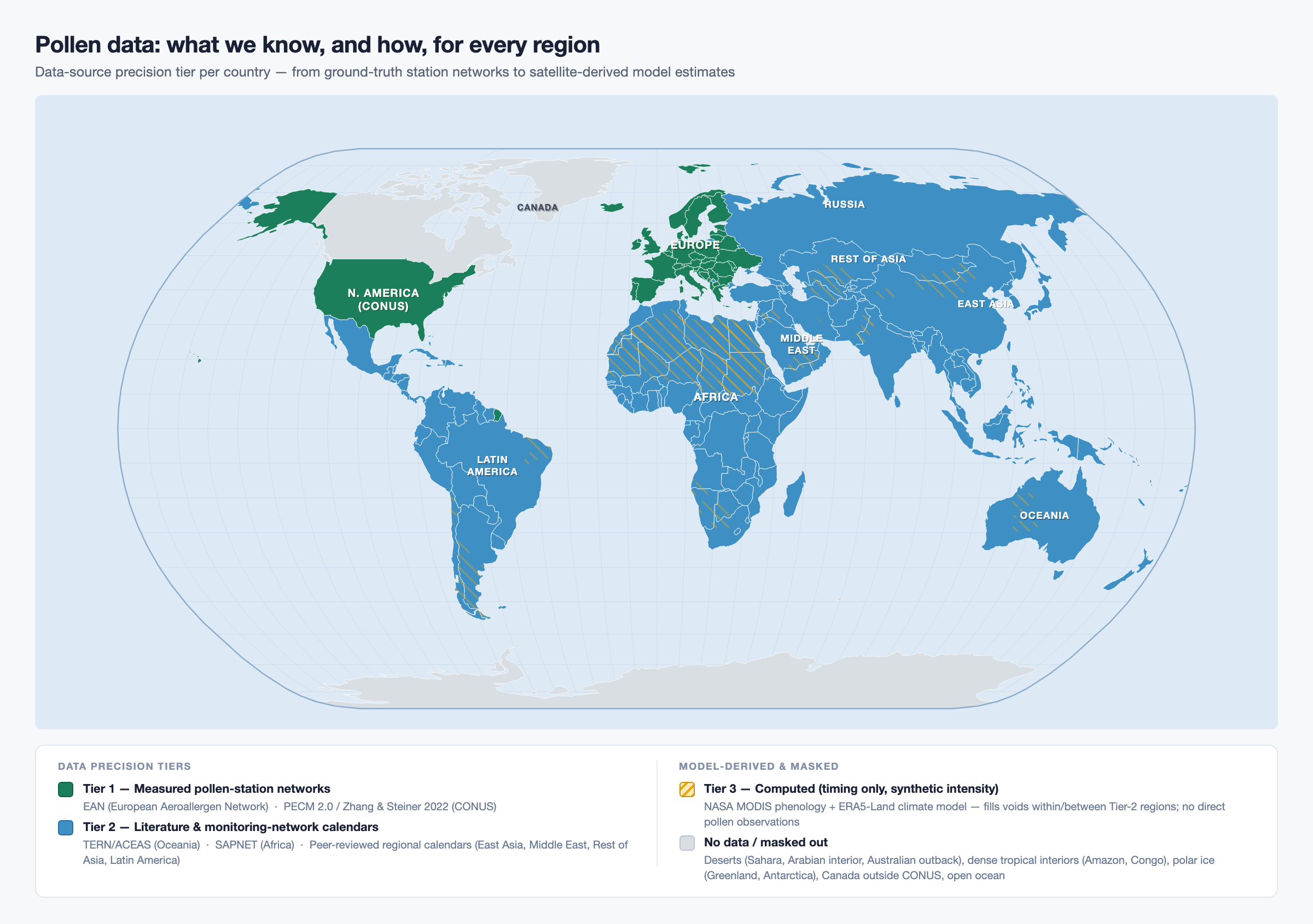
Pollen data sources by region — measured (green), literature (blue), model-computed (amber), masked (grey)

At a glance: green regions are measured station networks, blue are literature/network calendars, amber is the computed timing-only model, and grey is masked out (no defensible estimate). The rest of this post digs into how the blue and amber tiers are built.

Digging deeper: how the rest of the map is computed

Outside the two measured anchors, the map is built by re-computing and imputing the season — interpolating sparse calendars and, where even that runs out, modelling timing from satellite and climate data. Everything below follows from one honest constraint.

The one rule: claim WHEN, never HOW MUCH

The whole design follows from a single honest constraint. Where we have real measurements (Europe, North America, East Asia, Oceania), the map shows interpolated measured / literature pollen levels. Everywhere else, a satellite-and-climate model fills the gaps — but it only claims the season window (roughly when a taxon flowers), never the intensity. Satellite greenness correlates with airborne-pollen concentration at Spearman ρ ≈ 0 [rank correlation ≈ zero], so modelled areas get a single flat, conservative in-season level, sit in the lower confidence tiers, are aggressively masked where indefensible, and carry a visible confidence indicator. That honesty is the methodology.

Two composition guarantees hold everywhere:

Override-never-overwrite — the model only fills confirmed no-data voids; real and literature data are byte-verified to never change (0 pre-existing data pixels altered in every region apply).
Honest masking — where no defensible estimate exists (Sahara, Amazon/Congo interior, ice, ocean), the pixel stays transparent. Africa masks 84.3% of its voids; Oceania 99.2%.

End-to-end pipeline

Three source pipelines feed one on-disk format, which feeds the WebGL app. (See the two data branches for how measured and modelled data compose.)

graph LR;
  S1[Measured pollen stations]:::real --> T1[IDW spatial interpolation];
  S2[Literature pollen calendars]:::real --> T1;
  S3[NASA MODIS plus ERA5-Land climate]:::model --> T2[B0 void-fill model];
  T1 --> M[Override-never-overwrite merge];
  T2 --> M;
  M --> E[Encoding-B PNG atlas];
  M --> C[conf.png confidence raster];
  E --> APP[WebGL world map];
  C --> APP;
  classDef real fill:#1a7f5a,color:#fff;
  classDef model fill:#e6a817,color:#3a2a00;

Two branches, one merge

The left branch carries real signal; the right branch is the global model. Both emit identical Encoding-B strips, then merge in priority order so the model only shows through where nothing better exists.

graph TD;
  A[Measured stations Hirst-trap counts]:::real --> B[IDW interpolation per region];
  A2[Peer-reviewed pollen calendars]:::real --> B;
  B --> MERGE{Compose higher tier wins};
  D[NASA MODIS plus ESA WorldCover plus ERA5-Land]:::model --> E[B0 void-fill model];
  E --> A4[A4 quality-floor mask];
  A4 --> MERGE;
  MERGE --> OUT[Encoding-B level strips];
  MERGE --> CONF[conf.png per-pixel tier];
  classDef real fill:#1a7f5a,color:#fff;
  classDef model fill:#e6a817,color:#3a2a00;

Inside the B0 model

The void-fill model (we call it the B0 model [satellite+climate void-filler]) ingests NASA MODIS phenology (MCD12Q2 greenup) [satellite green-up timing] and MODIS land cover (MCD12Q1) [plant functional types] from NASA Earthdata, plus ERA5-Land 2 m air temperature from the Copernicus Climate Data Store. It derives a per-taxon flowering onset via three paths, then sets a flat conservative intensity. Crucially, growing-degree-day accumulation starts from each pixel’s local thermal-year origin (its coldest week), so the Southern Hemisphere is seasonally correct by construction — no hemisphere-flip hack anywhere.

graph TD;
  G[MODIS MCD12Q2 greenup DOY]:::in --> PA[Path A: greenup plus per-taxon offset];
  T[ERA5-Land 2m temperature]:::in --> PB[Path B: GDD from local thermal-year origin];
  L[MODIS MCD12Q1 land cover]:::in --> RANGE[Range and PFT gating];
  PC[Path C: fixed-photoperiod weeds AMBR ARTE]:::in --> ONSET[Per-taxon flowering onset];
  PA --> ONSET;
  PB --> ONSET;
  ONSET --> FLAT[Flat conservative intensity capped at level 2];
  RANGE --> FLAT;
  FLAT --> Z[Calibrated season window];
  classDef in fill:#e6a817,color:#3a2a00;

Path A — trees & grass (primary): onset = MODIS greenup + a per-taxon offset.
Path B — GDD fallback [growing-degree-day thermal model]: used where phenology QA is poor; accumulates heat from the pixel’s local coldest week, thresholds frozen to priors.
Path C — photoperiod weeds: ragweed (AMBR) [Ambrosia] and mugwort (ARTE) [Artemisia] flower on a fixed solstice-relative photoperiod, so they are hemisphere-aware by definition.

Intensity is a single per-taxon constant taken from the Europe + North America median (e.g. EU grass in-season mean ≈ 2.04 → level 2) — a flat plateau, not a per-pixel gradient and not a bell curve.

Calibration is the whole point

The model is fit and validated against the decoded real ordinal data for Europe and North America — the precision anchors. The test is timing, not intensity.

Test	Method	Gate	Result
Onset / peak timing	Spatial k-fold cross-validation on EU+NA, held-out	onset ≤ 3 wk, peak ≤ 3 wk	11 / 17 taxa pass [taxa = pollen types]
Cross-region transfer	EU ↔ NA peak-week transfer	cross-region peak ≤ 4 wk	gated together with above
Literature cross-check (K-LIT)	Family peak vs published regional calendar	within ± 4 wk	AMBR + ARTE only, in LatAm + Middle East
Intensity	satellite greenness vs airborne pollen	(retired)	ρ ≈ 0 → flat constant instead

Two consequences make the honesty concrete. First, the most universal allergen — grasses (POAC [Poaceae]) — flips PASS→FAIL on held-out data (onset/peak error 3.4 / 3.2 wk, just past the ≤ 3.0 wk gate), so grass ships synthetic everywhere in the void-fill. Second, the literature cross-check (K-LIT) is the only test inside the true extrapolation domain (arid / tropical / Southern Hemisphere), and only AMBR + ARTE clear it — which is why the entire model tier is just ragweed + mugwort in two regions. Everything else that survives masking is synthetic.

The confidence ladder

Every pixel carries one of five tiers, recorded in a separate conf.png raster that reuses the same byte ladder as the level strips (the two rasters share the numbers {0,64,…} but must not be conflated). A higher tier always wins the merge.

graph LR;
  M255[Measured byte 255 station IDW]:::t1 --> L192[Literature byte 192 pollen calendars]:::t2;
  L192 --> MO128[Model byte 128 K-LIT-anchored season]:::t3;
  MO128 --> S64[Synthetic byte 64 biological-prior season]:::t4;
  S64 --> N0[No-data byte 0 masked transparent]:::t5;
  classDef t1 fill:#1a7f5a,color:#fff;
  classDef t2 fill:#3d8fc4,color:#fff;
  classDef t3 fill:#e6a817,color:#3a2a00;
  classDef t4 fill:#c46e2d,color:#fff;
  classDef t5 fill:#c0c0c0,color:#333;

The Encoding-B format

Each taxon ships as 4 PNG strips × 13 weekly slices = 52 ISO weeks, grayscale-8, with bytes drawn from a 5-value ladder {0, 64, 128, 192, 255} mapping to pollen levels 0–4. Composition happens at extraction time, so the PNG already encodes the merged result — the app just samples it.

graph LR;
  TAX[One taxon for one region]:::h --> ST[4 PNG strips];
  ST --> SL[13 weekly slices each];
  SL --> W[52 ISO weeks total];
  W --> BYTE[Byte ladder 0 64 128 192 255];
  BYTE --> LV[Levels 0 1 2 3 4 none to very high];
  classDef h fill:#3d8fc4,color:#fff;

The eight regions

All facts below are read directly from each region’s shipped manifest (region, dims, nAllergens, confidence/confidenceFloor, provenance.sources). The 52-week temporal structure is fixed by the Encoding-B format (confirmed in the app and methodology, not stored as a manifest field). Europe and North America carry no tier field in their manifest — they are the highest-quality measured anchors and are described qualitatively below.

Region	Grid (W×H)	Taxa	Weeks	Dominant tier	Primary data source · license
Europe	600×800	12	52	Measured (anchor; no tier field)	EAN climatology via polleninformation.at · © 2012 EAN
North America (CONUS)	585×260	13	52	Measured (anchor; no tier field)	PECM 2.0 (Zhang & Steiner 2022) · CC BY 4.0
Korea + Japan (East Asia)	440×320	14	52	Literature → IDW (no tier field)	Open-access EA pollen literature · CC BY / equiv.
Oceania (AU & NZ)	838×488	13	52	Literature (floor: synthetic)	TERN / ACEAS network · CC BY 4.0
Middle East	410×406	14	52	Literature (floor: synthetic)	Qatar PLoS ONE + Turkey calendars · CC BY 4.0
Rest of Asia	640×730	20	52	Literature (floor: synthetic)	China/Pakistan/SE-Asia/Russia studies · CC BY 4.0
Latin America	989×1048	17	52	Literature (floor: synthetic)	Santiago, Chile (Toro 2015) · CC BY 4.0
Africa	1014×987	12	52	Literature (floor: synthetic)	SAPNET (7 cities) · CC BY 4.0

The five fill regions are dominantly literature but floor at synthetic because their void-fill is mostly biological-prior. Verified void-fill outcomes from the apply reports: Middle East 7,605 voids filled (8.2%, 91.8% masked, ARTE the only model-tier taxon); Asia-rest 163,985 (41.6%, 58.4% masked, zero model pixels); Oceania 2,806 (0.76%, 99.2% masked, zero model); Africa 149,309 (15.68%, 84.32% masked, zero model); Latin America 366,106 voids filled with just 8 model pixels (AMBR/ARTE within 5° of a Southern-Hemisphere anchor). Africa, Oceania and Asia-rest have zero model pixels — the entire model tier is AMBR + ARTE in two regions.

Explore it yourself on the interactive map →

Data & sources

Here is everything the map draws on, grouped by what it does. Attribution strings are reproduced verbatim from the region manifests.

Measured pollen data

Europe — EAN climatology. Pollen-load climatology published as the ContaminationMapEurope widget on polleninformation.at, produced with the European Aeroallergen Network (EAN), Medical University of Vienna (© 2012 EAN).
North America (CONUS) — PECM 2.0 (CC BY 4.0). Pollen-emission climatology, 1995–2014 historical average. Zhang & Steiner (2022, Nature Communications, doi:10.1038/s41467-022-28764-0). Data: doi:10.7302/628t-r416.

Literature & network pollen data

Oceania — TERN / ACEAS (CC BY 4.0). Pollen monitoring network (portal.tern.org.au), 9 AU/NZ stations.
Africa — SAPNET (CC BY 4.0). Two-year South African pollen monitoring network report (PMC10620116), 7 cities, 2019–2021.
Middle East (CC BY 4.0). Qatar / Arabian Peninsula calendar, PLoS ONE 2022, doi:10.1371/journal.pone.0270975; Turkey NE Anatolia (Posof/Ardahan), Scientific Reports 2025, doi:10.1038/s41598-025-05867-4; Turkey SE Anatolia (Siirt), Biology 14(7):841, 2025, doi:10.3390/biology14070841.
Latin America (CC BY 4.0). Toro et al. (2015, PLoS ONE, doi:10.1371/journal.pone.0123077), Santiago, Chile.
East Asia & rest of Asia. Open-access regional pollen-calendar literature (China / Korea / Japan / Pakistan / SE-Asia / Russia studies), CC BY or equivalent.

Satellite & climate inputs

NASA MODIS MCD12Q2 V061 [satellite green-up timing] (LP DAAC): Friedl, Gray & Sulla-Menashe (2022), doi:10.5067/MODIS/MCD12Q2.061.
NASA MODIS MCD12Q1 V061 [satellite land cover] (LP DAAC): Friedl & Sulla-Menashe (2022), doi:10.5067/MODIS/MCD12Q1.061.
ERA5-Land (Copernicus Climate Change Service): “Generated using Copernicus Climate Change Service information [1950–2024]. ERA5-Land monthly averaged data from 1950 to present (doi:10.24381/cds.e2161bac). Neither the European Commission nor ECMWF is responsible for any use that may be made of the Copernicus information or data it contains.”
ESA WorldCover 2021 v200 (CC BY 4.0): “© ESA WorldCover project 2021 / Contains modified Copernicus Sentinel data (2021) processed by ESA WorldCover consortium.”
WorldClim 2.1: Fick & Hijmans (2017), Int. J. Climatology 37(12):4302–4315, doi:10.1002/joc.5086.
GALORE global modern pollen (CC BY 4.0): Pound & O’Keefe (2024), doi:10.5281/zenodo.14161411 — pipeline-internal range-gate prior only.
GBIF species occurrences (CC BY 4.0): per-download DOI — pipeline-internal range-gate prior only.

Basemap & reference

Basemap tiles by OpenFreeMap (OpenMapTiles schema), © OpenStreetMap contributors; land mask from Natural Earth (public domain).

Not endorsed by ESA, Copernicus/ECMWF, NASA, TERN, SAPNET, PLoS ONE, or any data provider. This is a research project explaining a modelled product — the void-fill claims a season window and presence at the stated confidence tier, never a measured pollen concentration.